case(+Template, +Tuples, +Dag)case(+Template, +Tuples, +Dag, +Options)This constraint encodes an n-ary constraint, defined by extension and/or linear inequalities. It uses a DAG-shaped data structure where nodes corresponds to variables and every arc is labeled by an admissible interval for the node above it and optionally by linear inequalities. The variable order is fixed: every path from the root node to a leaf node should visit every variable exactly once, in the order in which they occur lexically in Template. The constraint is true for a single ground tuple if there is a path from the root node to a leaf node such that (a) each tuple element is contained in the corresponding Min..Max interval on the path, and (b) any encountered linear inequalities along the path are true.
The case constraint is true for a set of ground tuples if it is
true for each tuple of the set. The details are given below.
Template is a nonground Prolog term, each variable of which should occur exactly once. Its variables are merely place-holders; they should not occur outside the constraint nor inside Tuples.
Tuples is a list of terms of the same shape as Template. They should not share any variables with Template.
Dag is a list of nodes of the form
node(ID,X,Children), where X is a
template variable, and ID should be an integer, uniquely
identifying each node. The first node in the list is the root
node.
Nodes are either internal nodes or leaf nodes. For an
internal node, Children is a list of terms
(Min..Max)-ID2 or
(Min..Max)-SideConstraints-ID2, where
ID2 is the ID of a child node, Min is an integer or the atom
inf (minus infinity), and Max is an integer or the atom
sup (plus infinity). For a leaf node, Children is a list
of terms (Min..Max) or
(Min..Max)-SideConstraints.
SideConstraints is a list of side constraints of the form
scalar_product(Coeffs, Xs, #=<, Bound), where
Coeffs is a list of length k of integers, Xs is a list
of length k of template variables, and Bound is an integer.
Variables in Tuples for which their template variable counterparts are constrained by side constraints, must have bounded domains. In the absence of side constraint, the constraint maintains domain consistency.
The use of side constraint is deprecated, because the level of consistency is no better than the alternative, namely to use separate, reified arithmetic constraints and possibly auxiliary variables.
Options is a list of zero or more of the following:
scalar_product(Coeffs, Xs, #=<, Bound) since release 4.2,deprecated-
A side constraint located at the root of the DAG.
For example, recall that element(X,L,Y) wakes
up when the domain of X or the lower or upper bound of Y has
changed, performs full pruning of X, but only prunes the bounds of
Y. The following two constraints:
element(X, [1,1,1,1,2,2,2,2], Y),
element(X, [10,10,20,20,10,10,30,30], Z)
can be replaced by the following single constraint, which is equivalent declaratively, but which maintains domain consistency:
elts(X, Y, Z) :-
    case(f(A,B,C), [f(X,Y,Z)],
         [node(0, A,[(1..2)-1,(3..4)-2,(5..6)-3,(7..8)-4]),
          node(1, B,[(1..1)-5]),
          node(2, B,[(1..1)-6]),
          node(3, B,[(2..2)-5]),
          node(4, B,[(2..2)-7]),
          node(5, C,[(10..10)]),
          node(6, C,[(20..20)]),
          node(7, C,[(30..30)])]).
The DAG of the previous example has the following shape:
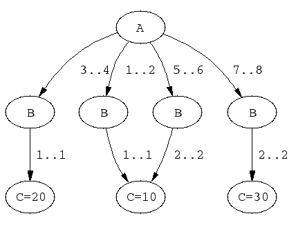
elts/3.
A couple of sample queries:
| ?- elts(X, Y, Z).
X in 1..8,
Y in 1..2,
Z in {10}\/{20}\/{30}

| ?- elts(X, Y, Z), Z #>= 15.
X in(3..4)\/(7..8),
Y in 1..2,
Z in {20}\/{30}

| ?- elts(X, Y, Z), Y = 1.
Y = 1,
X in 1..4,
Z in {10}\/{20}
As an example with side constraints, consider assigning tasks to machines with given unavailibility periods. In this case, one can use a calendar constraint [CHIP 03, Beldiceanu, Carlsson & Rampon 05] to link the real origins of the tasks (taking the unavailibility periods into account) with virtual origins of the tasks (not taking the unavailibility periods into account). One can then state machine resource constraints using the virtual origins, and temporal constraints between the tasks using the real origins.
Assume, for example, three machines with unavailibility periods given by the following table:
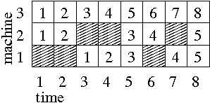
Machine 1 is not available during (real) time periods 1-2
and 6-6, machine 2 is not available during (real) time
periods 3-4 and 7-7, and machine 3 is always
available.
The following can then be used to express a calendar constraint for a
given task scheduled on machine M in 1..3, with virtual
origin V in 1..8, and real origin R in 1..8:
calendar(M, V, R) :-
        M in 1..3,
        V in 1..8,
        R in 1..8,
        smt((M#=1 #/\ V in 1..3 #/\ R#=V+2) #\/
            (M#=1 #/\ V in 4..5 #/\ R#=V+3) #\/
            (M#=2 #/\ V in 1..2 #/\ R#=V) #\/
            (M#=2 #/\ V in 3..4 #/\ R#=V+2) #\/
            (M#=2 #/\ V in 5..5 #/\ R#=V+3) #\/
            (M#=3               #/\ R#=V)).
or equivalently as:
calendar(M, V, R) :-
    case(f(A,B,C),
         [f(M,V,R)],
         [node(0, A, [(1..1)-1, (2..2)-2, (3..3)-3]),
          node(1, B, [(1..3)-[scalar_product([1,-1],[B,C],#=<,-2),
                              scalar_product([1,-1],[C,B],#=<, 2)]-4,
                      (4..5)-[scalar_product([1,-1],[B,C],#=<,-3),
                              scalar_product([1,-1],[C,B],#=<, 3)]-4]),
          node(2, B, [(1..2)-[scalar_product([1,-1],[B,C],#=<, 0),
                              scalar_product([1,-1],[C,B],#=<, 0)]-4,
                      (3..4)-[scalar_product([1,-1],[B,C],#=<,-2),
                              scalar_product([1,-1],[C,B],#=<, 2)]-4,
                      (5..5)-[scalar_product([1,-1],[B,C],#=<,-3),
                              scalar_product([1,-1],[C,B],#=<, 3)]-4]),
          node(3, B, [(1..8)-[scalar_product([1,-1],[B,C],#=<, 0),
                              scalar_product([1,-1],[C,B],#=<, 0)]-4]),
          node(4, C, [(1..8)])]).
Note that equality must be modeled as the conjunction of inequalities,
as only constraints of the form scalar_product(+Coeffs,
+Xs, #=<, +Bound) are allowed as side constraints.
The DAG of the calendar constraint has the following shape:
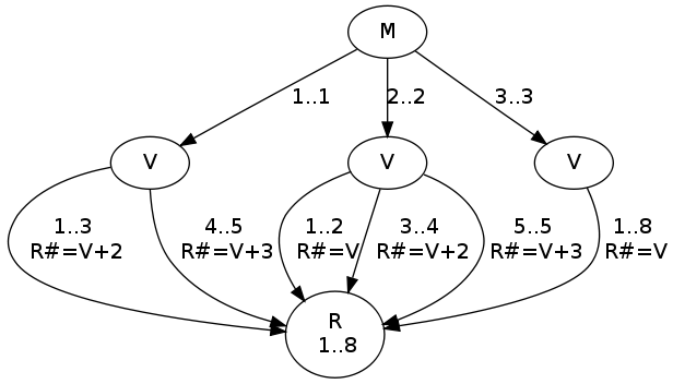
calendar/3.
A couple of sample queries:
| ?- M in 1..3, V in 1..8, R in 1..8,
     calendar(M, V, R).
M in 1..3,
V in 1..8,
R in 1..8

| ?- M in 1..3, V in 1..8, R in 1..8,
     calendar(M, V, R), M #= 1.
M = 1,
V in 1..5,
R in 1..8

| ?- M in 1..3, V in 1..8, R in 1..8,
     calendar(M, V, R), M #= 2, V #> 4.
M = 2,
V = 5,
R = 8