10.34.3.4 Combinatorial Constraints

The constraints listed here are sometimes called symbolic constraints. They are currently not reifiable. Unless documented otherwise, they maintain (at most) bound-consistency in their arguments; see The Constraint System.

global_cardinality(+Xs,+Vals)
global_cardinality(+Xs,+Vals,+Options)
where Xs = [X_1,\ldots,X_d] is a list of integers or domain variables, and Vals = [K_1-V_1,\ldots,K_n-V_n] is a list of pairs where each key K_i is a unique integer and V_i is a domain variable or an integer. True if every element of Xs is equal to some key and for each pair K_i-V_i, exactly V_i elements of Xs are equal to K_i.

If either Xs or Vals is ground, and in many other special cases, global_cardinality/[2,3] maintains arc-consistency, but generally, bound-consistency cannot be guaranteed. An arc-consistency algorithm [Regin 96] is used, roughly linear in the total size of the domains.

Options is a list of zero or more of the following:

consistency(Cons)
Which filtering algorithm to use. One of the following:
domain
The constraint will use the algorithm mentioned above. Implies on(dom). The default.
bound
The constraint will use the algorithm mentioned above. Implies on(minmax).
value
The constraint will use a simple algorithm, which prevents too few or too many of the Xs from taking values among the Vals. Implies on(val).

on(On)
How eagerly to wake up the constraint. One of the following:
dom
to wake up when the domain of a variable is changed (the default);
minmax
to wake up when the domain bound of a variable is changed;
val
to wake up when a variable becomes ground.

cost(Cost,Matrix)
Overrides any consistency/1 option value. A cost is associated with the constraint and reflected into the domain variable Cost. Matrix should be a d\times n matrix, represented as a list of d lists, each of length n. Assume that each X_i equals K_(p_i). The cost of the constraint is then \Matrix[1,p_1]+\cdots+\Matrix[d,p_d].

With this option, an arc-consistency algorithm [Regin 99] is used, the complexity of which is roughly O(d(m + n \log n)) where m is the total size of the domains.


element(?X,+List,?Y)
where X and Y are integers or domain variables and List is a list of integers or domain variables. True if the X:th element of List is Y. Operationally, the domains of X and Y are constrained so that for every element in the domain of X, there is a compatible element in the domain of Y, and vice versa.

Maintains arc-consistency in X and bound-consistency in List and Y. Corresponds to nth1/3 in library(lists).

table(+Tuples,+Extension)
table(+Tuples,+Extension,+Options)
Defines an n-ary constraint by extension. Extension should be a set of lists of integers, each of length n. Tuples should be a set of lists of domain variables or integers, each also of length n. The constraint holds if every Tuple in Tuples occurs in the Extension.

For convenience, Extension may contain ConstantRange (see Syntax of Indexicals) expressions in addition to integers.

Options is a list of zero or more of the following. It can be used to control the waking and pruning conditions of the constraint:

consistency(Cons)
The value is one of the following:
domain
The constraint will maintain arc-consistency (the default).
bound
The constraint will maintain bound-consistency.
value
The constraint will wake up when a variable has become ground, and only prune a variables when its domain has been reduced to a singleton.

table/[2,3] is implemented in terms of the following, more general constraint, with which arbitrary relations can be defined compactly:

case(+Template, +Tuples, +Dag)
case(+Template, +Tuples, +Dag, +Options)

Template is an arbitrary non-ground Prolog term. Its variables are merely place-holders; they should not occur outside the constraint nor inside Tuples.

Tuples is a list of terms of the same shape as Template. They should not share any variables with Template.

Dag is a list of nodes of the form node(ID,X,Successors), where X is a place-holder variable. The set of all X should equal the set of variables in Template. The first node in the list is the root node. Let rootID denote its ID.

Nodes are either internal nodes or leaf nodes. In the former case, Successors is a list of terms (Min..Max)-ID2, where the ID2 refers to a child node. In the latter case, Successors is a list of terms (Min..Max). In both cases, the (Min..Max) should form disjoint intervals.

ID is a unique, integer identifier of a node.

Each path from the root node to a leaf node corresponds to one set of tuples admitted by the relation expressed by the constraint. Each variable in Template should occur exactly once on each path, and there must not be any cycles.

Options is a list of zero or more of the following. It can be used to control the waking and pruning conditions of the constraint, as well as to identify the leaf nodes reached by the tuples:

leaves(TLeaf,Leaves)
TLeaf is a place-holder variable. Leaves is a list of variables of the same length as Tuples. This option effectively extends the relation by one argument, corresponding to the ID of the leaf node reached by a particular tuple.
on(Spec)
Specifies how eagerly the constraint should react to domain changes of X.
prune(Spec)
Specifies the extent to which the constraint should prune the domain of X.

Spec is one of the following, where X is a place-holder variable occurring in Template or equal to TLeaf:

dom(X)
wake up when the domain of X has changed, resp. perform full pruning on X. This is the default for all variables mentioned in the constraint.
min(X)
wake up when the lower bound of X has changed, resp. prune only the lower bound of X.
max(X)
wake up when the upper bound of X has changed, resp. prune only the upper bound of X.
minmax(X)
wake up when the lower or upper bound of X has changed, resp. prune only the bounds of X.
val(X)
wake up when X has become ground, resp. only prune X when its domain has been reduced to a singleton.
none(X)
ignore domain changes of X, resp. never prune X.

The constraint holds if path(rootID,Tuple,Leaf) holds for each Tuple in Tuples and Leaf is the corresponding element of Leaves if given (otherwise, Leaf is a free variable).

path(ID,Tuple,Leaf) holds if Dag contains a term node(ID,Var,Successors), Var is the unique k:th element of Template, i is the k:th element of Tuple, and:

For example, recall that element(X,L,Y) wakes up when the domain of X or the lower or upper bound of Y has changed, performs full pruning of X, but only prunes the bounds of Y. The following two constraints:

          element(X, [1,1,1,1,2,2,2,2], Y),
          element(X, [10,10,20,20,10,10,30,30], Z)
     

can be replaced by the following single constraint, which is equivalent declaratively as well as wrt. pruning and waking. The fourth argument illustrates the leaf feature:
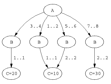
          elts(X, Y, Z, L) :-
              case(f(A,B,C), [f(X,Y,Z)],
                   [node(0, A,[(1..2)-1,(3..4)-2,(5..6)-3,(7..8)-4]),
                    node(1, B,[(1..1)-5]),
                    node(2, B,[(1..1)-6]),
                    node(3, B,[(2..2)-5]),
                    node(4, B,[(2..2)-7]),
                    node(5, C,[(10..10)]),
                    node(6, C,[(20..20)]),
                    node(7, C,[(30..30)])],
                   [on(dom(A)),on(minmax(B)),on(minmax(C)),
                    prune(dom(A)),prune(minmax(B)),prune(minmax(C)),
                    leaves(_,[L])]).
     

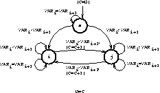
The DAG of the previous example has the following shape:


images/clpfd1.png
DAG corresponding to elts/4

A couple of sample queries:

          | ?- elts(X, Y, Z, L).
          L in 5..7,
          X in 1..8,
          Y in 1..2,
          Z in 10..30
          
          | ?- elts(X, Y, Z, L), Z #>= 15.
          L in 6..7,
          X in(3..4)\/(7..8),
          Y in 1..2,
          Z in 20..30
          
          | ?- elts(X, Y, Z, L), Y = 1.
          Y = 1,
          L in 5..6,
          X in 1..4,
          Z in 10..20
          
          | ?- elts(X, Y, Z, L), L = 5.
          Z = 10,
          X in(1..2)\/(5..6),
          Y in 1..2
     

all_different(+Variables)
all_different(+Variables, +Options)
all_distinct(+Variables)
all_distinct(+Variables, +Options)
where Variables is a list of domain variables or integers. Each variable is constrained to take a value that is unique among the variables. Declaratively, this is equivalent to an inequality constraint for each pair of variables.

Options is a list of zero or more of the following:

consistency(Cons)
Which algorithm to use, one of the following:
domain
The default for all_distinct/[1,2] and assignment/[2,3]. an arc-consistency algorithm [Regin 94] is used, roughly linear in the total size of the domains. Implies on(dom).
bound
a bound-consistency algorithm [Mehlhorn 00] is used. This algorithm is nearly linear in the number of variables and values. Implies on(minmax).
value
The default for all_different/[1,2]. An algorithm achieving exactly the same pruning as a set of pairwise inequality constraints is used, roughly linear in the number of variables. Implies on(val).

on(On)
How eagerly to wake up the constraint. One of the following:
dom
(the default for all_distinct/[1,2] and assignment/[2,3]), to wake up when the domain of a variable is changed;
min
to wake up when the lower bound of a domain is changed;
max
to wake up when the upper bound of a domain is changed;
minmax
to wake up when some bound of a domain is changed;
val
(the default for all_different/[1,2]), to wake up when a variable becomes ground.

nvalue(?N, +Variables)
where Variables is a list of domain variables with finite bounds or integers, and N is an integer or a domain variable. True if N is the number of distinct values taken by Variables. Approximates bound-consistency in N and arc-consistency in Variables. Can be thought of as a relaxed version of all_distinct/2.

The following is a constraint over two lists of length n of variables. Each variable is constrained to take a value in [1,n] that is unique for its list. Furthermore, the lists are dual in a sense described below.

assignment(+Xs, +Ys)
assignment(+Xs, +Ys, +Options)
where Xs = [X_1,\ldots,X_n] and Ys = [Y_1,\ldots,Y_n] are lists of domain variables or integers. True if all X_i, Y_i \in [1,n] and X_i=j \equiv Y_j=i.

Options is a list of zero or more of the following, where Boolean must be true or false (false is the default):

on(On)
Same meaning as for all_different/2.
consistency(Cons)
Same meaning as for all_different/2.
circuit(Boolean)
If true, circuit(Xs,Ys) must hold for the constraint to be true.
cost(Cost,Matrix)
A cost is associated with the constraint and reflected into the domain variable Cost. Matrix should be an n\times n matrix, represented as a list of lists. The cost of the constraint is \Matrix[1,X_1]+\cdots+\Matrix[n,X_n].

With this option, an arc-consistency algorithm [Sellmann 02] is used, the complexity of which is roughly O(n(m + n \log n)) where m is the total size of the domains.

The following constraint can be thought of as constraining n nodes in a graph to form a Hamiltonian circuit. The nodes are numbered from 1 to n. The circuit starts in node 1, visits each node, and returns to the origin.

circuit(+Succ)
circuit(+Succ, +Pred)
where Succ is a list of length n of domain variables or integers. The i:th element of Succ (Pred) is the successor (predecessor) of i in the graph. True if the values form a Hamiltonian circuit.

The following constraint can be thought of as constraining n tasks so that the total resource consumption does not exceed a given limit at any time:

cumulative(+Tasks)
cumulative(+Tasks,+Options)

A task is represented by a term task(O_i,D_i,E_i,H_i,T_i) where O_i is the start time, D_i the non-negative duration, E_i the end time, H_i the non-negative resource consumption, and T_i the task identifier. All fields are domain variables with bounded domains, or integers.

Let L be a global resource limit (by default 1, but see below), and:

          a = min(S1,...,Sn),
          b = max(S1+D1,...,Sn+Dn)
          Rij = Rj, if Sj =< i < Sj+Dj
          Rij = 0 otherwise
     

The constraint holds if:

  1. For every task i, Si+Di=Ei.
  2.                Ri1+...+Rin =< L, for all a =< i < b
              

Options is a list of zero or more of the following, where Boolean must be true or false (false is the default, except for the bounds_only option):

limit(L)
See above.
precedences(Ps)
Ps encodes a set of precedence constraints to apply to the tasks. Ps should be a list of terms of the form
               Ti-Tj #= Dij
          

where Ti and Tj should be task identifiers, and Dij should be a a domain variable (or an integer), denoting:

               S_i-S_j = D_ij \land D_ij \in r
          

global(Boolean)
if true, a more expensive algorithm will be used in order to achieve tighter pruning of the bounds of the parameters.

This constraint is due to Aggoun and Beldiceanu [Aggoun & Beldiceanu 93].

The following constraint can be thought of as constraining n tasks to be placed in time and on m machines. Each machine has a resource limit, which is interpreted as a lower or upper bound on the total amount of resource used on that machine at any point in time that intersects with some task.

cumulatives(+Tasks,+Machines)
cumulatives(+Tasks,+Machines,+Options)

A task is represented by a term task(O_i,D_i,E_i,H_i,M_i) where O_i is the start time, D_i the duration, E_i the end time, H_i the resource consumption, and M_i a machine identifier.

A machine is represented by a term machine(M_j,L_j) where M_j is the identifier and L_j is the resource limit of the machine.

All fields are domain variables with bounded domains, or integers. L_j must be an integer. D_i must be non-negative, but H_i may be either positive or negative. Negative resource consumption is interpreted as resource production.

Options is a list of zero or more of the following, where Boolean must be true or false (false is the default):

bound(B)
If lower (the default), each resource limit is treated as a lower bound. If upper, each resource limit is treated as an upper bound.
prune(P)
If all (the default), the constraint will try to prune as many variables as possible. If next, only variables that occur in the first non-ground task term (wrt. the order given when the constraint was posted) can be pruned.
generalization(Boolean)
If true, extra reasoning based on assumptions on machine assignment will be done to infer more.
task_intervals(Boolean)
If true, extra global reasoning will be performed in an attempt to infer more.

The following constraint captures the relation between a list of values, a list of the values in ascending order, and their positions in the original list:

sorting(+Xs,+Ps,+Ys)
where Xs = [X_1,\ldots,X_n], Ps = [P_1,\ldots,P_n], and Ys = [Y_1,\ldots,Y_n] are lists of domain variables or integers. The constraint holds if the following are true:

In practice, the underlying algorithm [Mehlhorn 00] is likely to achieve bound-consistency, and is guaranteed to do so if Ps is ground or completely free.

The following constraints model a set or lines or rectangles, respectively, so that no pair of objects overlap:

disjoint1(+Lines)
disjoint1(+Lines,+Options)
where Lines is a list of terms F(S_j,D_j) or F(S_j,D_j,T_j), S_j and D_j are domain variables with finite bounds or integers denoting the origin and length of line j respectively, F is any functor, and the optional T_j is an atomic term denoting the type of the line. T_j defaults to 0 (zero).

Options is a list of zero or more of the following, where Boolean must be true or false (false is the default):

decomposition(Boolean)
if true, an attempt is made to decompose the constraint each time it is resumed.
global(Boolean)
if true, a redundant algorithm using global reasoning is used to achieve more complete pruning.
wrap(Min,Max)
If used, the space in which the lines are placed should be thought of as a circle where positions Min and Max coincide, where Min and Max should be integers. That is, the space wraps around. Furthermore, this option forces the domains of the origin variables to be inside [Min,Max-1].
margin(T_1,T_2,D)
This option imposes a minimal distance D between the end point of any line of type T_1 and the origin of any line of type T_2. D should be a positive integer or sup. If sup is used, all lines of type T_2 must be placed before any line of type T_1.

This option interacts with the wrap/2 option in the sense that distances are counted with possible wrap-around, and the distance between any end point and origin is always finite.

The file library('clpfd/examples/bridge.pl') contains an example where disjoint1/2 is used for scheduling non-overlapping tasks.

disjoint2(+Rectangles)
disjoint2(+Rectangles,+Options)
where Rectangles is a list of terms F(S_(j_1),D_(j_1),S_(j_2),D_(j_2)) or F(S_(j_1),D_(j_1),S_(j_2),D_(j_2),T_j), S_(j_1) and D_(j_1) are domain variables with finite bounds or integers denoting the origin and size of rectangle j in the X dimension, S_(j_2) and D_(j_2) are the values for the Y dimension, F is any functor, and the optional T_j is an atomic term denoting the type of the rectangle. T_j defaults to 0 (zero).

Options is a list of zero or more of the following, where Boolean must be true or false (false is the default):

decomposition(Boolean)
If true, an attempt is made to decompose the constraint each time it is resumed.
global(Boolean)
If true, a redundant algorithm using global reasoning is used to achieve more complete pruning.
wrap(Min1,Max1,Min2,Max2)
Min1 and Max1 should be either integers or the atoms inf and sup respectively. If they are integers, the space in which the rectangles are placed should be thought of as a cylinder wrapping around the X dimension where positions Min1 and Max1 coincide. Furthermore, this option forces the domains of the S_(j_1) variables to be inside [Min1,Max1-1].

Min2 and Max2 should be either integers or the atoms inf and sup respectively. If they are integers, the space in which the rectangles are placed should be thought of as a cylinder wrapping around the Y dimension where positions Min2 and Max2 coincide. Furthermore, this option forces the domains of the S_(j_2) variables to be inside [Min2,Max2-1].

If all four are integers, the space is a toroid wrapping around both dimensions.

margin(T_1,T_2,D_1,D_2)
This option imposes minimal distances D_1 in the X dimension and D_2 in the Y dimension between the end point of any rectangle of type T_1 and the origin of any rectangle of type T_2. D_1 and D_2 should be positive integers or sup. If sup is used, all rectangles of type T_2 must be placed before any rectangle of type T_1 in the relevant dimension.

This option interacts with the wrap/4 option in the sense that distances are counted with possible wrap-around, and the distance between any end point and origin is always finite.

synchronization(Boolean)
Let the assignment dimension and the temporal dimension denote the two dimensions, no matter which is the X and which is the Y dimension. If Boolean is true, a redundant algorithm is used to achieve more complete pruning for the following case:
  • All rectangles have size 1 in the assignment dimension.
  • Some rectangles have the same origin and size in the temporal dimension, and that origin is not yet fixed.

The following example shows an artificial placement problem involving 25 rectangles including four groups of rectangles whose left and right borders must be aligned. If Synch is true, it can be solved with first-fail labeling in 23 backtracks. If Synch is false, 60 million backtracks do not suffice to solve it.

               ex([O1,Y1a,Y1b,Y1c,
                   O2,Y2a,Y2b,Y2c,Y2d,
                   O3,Y3a,Y3b,Y3c,Y3d,
                   O4,Y4a,Y4b,Y4c],
                  Synch) :-
                       domain([Y1a,Y1b,Y1c,
                               Y2a,Y2b,Y2c,Y2d,
                               Y3a,Y3b,Y3c,Y3d,
                               Y4a,Y4b,Y4c], 1, 5),
                       O1 in 1..28,
                       O2 in 1..26,
                       O3 in 1..22,
                       O4 in 1..25,
                       disjoint2([t(1,1,5,1),    t(20,4,5,1),
                                  t(1,1,4,1),    t(14,4,4,1),
                                  t(1,2,3,1),    t(24,2,3,1),
                                  t(1,2,2,1),    t(21,1,2,1),
                                  t(1,3,1,1),    t(14,2,1,1),
                                  t(O1,3,Y1a,1),
                                  t(O1,3,Y1b,1),
                                  t(O1,3,Y1c,1),
                                  t(O2,5,Y2a,1),
                                  t(O2,5,Y2b,1),
                                  t(O2,5,Y2c,1),
                                  t(O2,5,Y2d,1),
                                  t(O3,9,Y3a,1),
                                  t(O3,9,Y3b,1),
                                  t(O3,9,Y3c,1),
                                  t(O3,9,Y3d,1),
                                  t(O4,6,Y4a,1),
                                  t(O4,6,Y4b,1),
                                  t(O4,6,Y4c,1)],
                                 [synchronization(Synch)]).
          

The file library('clpfd/examples/squares.pl') contains an example where disjoint2/2 is used for tiling squares.

The following constraints express the fact that several vectors of domain variables are in ascending lexicographic order:

lex_chain(+Vectors)
lex_chain(+Vectors,+Options)
where Vectors is a list of vectors (lists) of domain variables with finite bounds or integers. The constraint holds if Vectors are in ascending lexicographic order.

Options is a list of zero or more of the following:

op(Op)
If Op is the atom #=< (the default), the constraints holds if Vectors are in non-descending lexicographic order. If Op is the atom #<, the constraints holds if Vectors are in strictly ascending lexicographic order.
increasing
This option imposes the additional constraint that each vector in Vectors be sorted in strictly ascending order.
among(Least,Most,Values)
If given, Least and Most should be integers such that 0 \leq \Least \leq \Most and Values should be a list of distinct integers. This option imposes the additional constraint on each vector in Vectors that at least Least and at most Most elements belong to Values.

Unless the increasing/0 or among/3 options are given, the underlying algorithm [Carlsson & Beldiceanu 02] guarantees arc-consistency.

The following constraint provides a general way of defining any constraint involving sequences whose checker, i.e. a procedure that classifies ground instances as solutions or non-solutions, can be expressed by a finite automaton, extended with counter operations on its arcs. The point is that it is very much easier to come up with such a checker that to come up with a filtering algorithm for the constraint of interest.

automaton(...)
The constraint has the form ctr according to the grammar shown below, which describes its abstract syntax. The arguments are:
sequence
The sequence of terms of interest.
template
A template for an item of the sequence. Only relevant if some state transition involving counter arithmetic mentions a variable occurring in template, in which case the corresponding term in a sequence element will be accessed.
signature
The signature of sequence. The automaton is not driven by the sequence itself, but by signature, which ranges over an alphabet, defined in the following argument. In addition to automaton/8, you must call a constraint that maps sequence to signature.
nodes
The nodes of the automaton, classified as source, sink or internal.
arcs
The arcs (transitions) of the automaton. Any transition not mentioned is assumed to go to an implicit failure node. An arc optionally contains expressions for updated counter values; by default, the counters remain unchanged. Conditional updates can be specified.
counters
For k counters, a list of k variables.
initial
For k counters, a list of k initial values, usually instantiated.
final
For k counters, a list of k final values, usually uninstantiated.

Abstract syntax:

ctr ::= automaton(sequence, template, signature,
nodes, arcs,
counters, initial, final)

sequence ::= list of template {all of which of the same shape}

template ::= term {most general shape of the sequence}
{its variables should be local to ctr}

signature ::= list of variable

nodes ::= list of nodespec {all of which of the same shape}

nodespec ::= source(node) {the initial state}
| sink(node) {an accept state}

node ::= atomic

arcs ::= list of arc {all of which of the same shape}

arc ::= arc(node,integer,node) {from node, integer, to node}
| arc(node,integer,node,exprs){exprs correspond to new counter values}
| arc(node,integer,node,conditional)

conditional ::= (cond -> exprs)
| (conditional ; conditional)

exprs ::= list of Expr {of same length as counters}
{Expr as defined in Syntax of Arithmetic Expressions}
{over counters, template and constants}
{variables occurring in counters correspond to old counter values}
{variables occurring in template refer to the current element of sequence}

cond ::= constraint {over counters, template and constants}
{must be reifiable or true}

counters ::= list of variable {should be local to ctr}

initial ::= list of integer {of same length as counters}

final ::= list of variable {of same length as counters}

If no counters are used, the arguments counters, initial and final should be []. The arguments template and sequence are only relevant if some Expr mentions a variable in template, in which case the corresponding position in sequence will be used at that point.

The constraint holds for a ground instance sequence if:

Here is an example. Suppose that you want to define the predicate inflexion(N,L) which should hold if L is a list of domain variables, and N is the number of times that the sequence order switches between strictly increasing and strictly decreasing. For example, the sequence [1,1,4,8,8,2,7,1] switches order three times.

Such a constraint is conveniently expressed by a finite automaton over the alphabet [<,=,>] denoting the order between consecutive list elements. A counter is incremented when the order switches, and is mapped to the first argument of the constraint. The automaton could look as follows:


images/inflexion2.png
Automaton for inflexion/2

The following piece of code encodes this using automaton/8. The auxiliary predicate inflexion_signature/2 maps the sequence to a signature where the consecutive element order is encoded over the alphabet [0,1,2]. We use one counter with initial value 0 and final value N (an argument of inflexion/2). Two transitions increment the counter. All states are accept states.

          inflexion(N, VARIABLES) :-
                  inflexion_signature(VARIABLES, SIGNATURE),
                  automaton(_, _, SIGNATURE,
                            [source(s),sink(i),sink(j),sink(s)],
                            [arc(s,1,s      ),
                             arc(s,2,i      ),
                             arc(s,0,j      ),
                             arc(i,1,i      ),
                             arc(i,2,i      ),
                             arc(i,0,j,[C+1]),
                             arc(j,1,j      ),
                             arc(j,0,j      ),
                             arc(j,2,i,[C+1])],
                            [C],[0],[N]).
          
          inflexion_signature([], []).
          inflexion_signature([_], []) :- !.
          inflexion_signature([VAR1,VAR2|VARs], [S|Ss]) :-
                  S in 0..2,
                  VAR1 #> VAR2 #<=> S #= 0,
                  VAR1 #= VAR2 #<=> S #= 1,
                  VAR1 #< VAR2 #<=> S #= 2,
                  inflexion_signature([VAR2|VARs], Ss).
     

A couple of queries:

          | ?- inflexion(N, [1,1,4,8,8,2,7,1]).
          N = 3 ? <RET>
          yes
          
          | ?- length(L,4), domain(L,0,1), inflexion(2,L), labeling([],L).
          L = [0,1,0,1] ? ;
          L = [1,0,1,0] ? ;
          no
     

This constraint was introduced in [Beldiceanu, Carlsson & Petit 04].


Send feedback on this subject.