10.35.3.4 Combinatorial Constraints

The constraints listed here are sometimes called symbolic constraints. They are currently not reifiable. Unless documented otherwise, they maintain (at most) bound-consistency in their arguments; see The Constraint System.

smt(:ConstraintBody)

The arithmetic, membership, and propositional constraints described earlier are transformed at compile time to conjunctions of library constraints. Although linear in the size of the source code, the expansion of a propositional formula over reifiable constraints to library goals can have time and memory overheads, and propagates disjunctions very weakly. Temporary variables holding intermediate values may have to be introduced, and the grain size of the constraint solver invocations can be rather small. As an alternative to the default propagation of such constraint formulas, this constraint is a front-end to the case/[3,4] propagator, which treats such a formula globally. The pruning can be stronger and it can run faster than the default propagator, but this is not necessarily the case. Bound-consistency is not guaranteed.

ConstraintBody should be of one of the following forms, or a propositional combination of such forms. See Syntax of Indexicals for the exact definition:


count(+Val,+List,+RelOp,?Count) deprecated
where Val is an integer, List is a list of integers or domain variables, Count an integer or a domain variable, and RelOp is a relational symbol as in Arithmetic Constraints. True if N is the number of elements of List that are equal to Val and N RelOp Count. Implemented by decomposition into one sum/3 constraint, one arithmetic comparison, and several reified equalities.

count/4 maintains arc-consistency, but in practice, the following constraint is a better alternative.

global_cardinality(+Xs,+Vals)
global_cardinality(+Xs,+Vals,+Options)
where Xs = [X1,...,Xd] is a list of integers or domain variables, and Vals = [K1-V1,...,Kn-Vn] is a list of pairs where each key Ki is a unique integer and Vi is a domain variable or an integer. True if every element of Xs is equal to some key and for each pair Ki-Vi, exactly Vi elements of Xs are equal to Ki.

If either Xs or Vals is ground, and in many other special cases, global_cardinality/[2,3] maintains arc-consistency, but generally, bound-consistency cannot be guaranteed. An arc-consistency algorithm [Regin 96] is used, roughly linear in the total size of the domains.

Options is a list of zero or more of the following:

consistency(Cons)
Which filtering algorithm to use. One of the following:
domain
The constraint will use the algorithm mentioned above. Implies on(dom). The default.
bound
The constraint will use the algorithm mentioned above. Implies on(minmax).
value
The constraint will use a simple algorithm, which prevents too few or too many of the Xs from taking values among the Vals. Implies on(val).

on(On)
How eagerly to wake up the constraint. One of the following:
dom
to wake up when the domain of a variable is changed (the default);
minmax
to wake up when the domain bound of a variable is changed;
val
to wake up when a variable becomes ground.

cost(Cost,Matrix)
Overrides any consistency/1 option value. A cost is associated with the constraint and reflected into the domain variable Cost. Matrix should be a d*n matrix of integers, represented as a list of d lists, each of length n. Assume that each Xi equals K(pi). The cost of the constraint is then Matrix[1,p1]+...+Matrix[d,pd].

With this option, an arc-consistency algorithm [Regin 99] is used, the complexity of which is roughly O(d(m + n log n)) where m is the total size of the domains.


element(?X,+List,?Y)
where X and Y are integers or domain variables and List is a list of integers or domain variables. True if the X:th element of List is Y. Operationally, the domains of X and Y are constrained so that for every element in the domain of X, there is a compatible element in the domain of Y, and vice versa.

Maintains arc-consistency in X and bound-consistency in List and Y. Corresponds to nth1/3 in library(lists).

relation(?X,+MapList,?Y) deprecated
where X and Y are integers or domain variables and MapList is a list of integer-ConstantRange pairs, where the integer keys occur uniquely (see Syntax of Indexicals). True if MapList contains a pair X-R and Y is in the range denoted by R.

An arbitrary binary constraint can be defined with relation/3. relation/3 is implemented by straightforward transformation to the following, more general constraint, with which arbitrary relations can be defined compactly:

table(+Tuples,+Extension)
table(+Tuples,+Extension,+Options)
Defines an n-ary constraint by extension. Extension should be a list of lists of integers, each of length n. Tuples should be a list of lists of domain variables or integers, each also of length n. The constraint holds if every Tuple in Tuples occurs in the Extension.

For convenience, Extension may contain ConstantRange (see Syntax of Indexicals) expressions in addition to integers.

Options is a list of zero or more of the following:

consistency(Cons)
This can be used to control the waking and pruning conditions of the constraint. The value is one of the following:
domain
The constraint will maintain arc-consistency (the default).
bound
The constraint will maintain bound-consistency.
value
The constraint will wake up when a variable has become ground, and only prune a variable when its domain has been reduced to a singleton.

nodes(Nb)
Nb is unified with the number of DAG nodes.
order(Order)
Determines the variable order of the DAG. The following values are valid:
leftmost
The order is the one given in the arguments (the default).
id3
Each tuple, and the columns of the extension, is permuted according to the heuristic that more discriminating columns should precede less discriminating ones.

method(Method)
Controls the way the DAG is generated from the extension, after permuting it if order(id3) was chosen. The following values are valid:
noaux
Equivalent DAG nodes are merged until no further merger is possible.
aux
An auxiliary, first variable is introduced, denoting extension row number. Then equivalent DAG nodes are merged until no further merger is possible.

table/[2,3] is implemented in terms of the following, more general constraint, with which arbitrary relations can be defined compactly:

case(+Template, +Tuples, +Dag)
case(+Template, +Tuples, +Dag, +Options)

This constraint encodes an n-ary constraint, defined by extension and/or linear inequalities. It uses a DAG-shaped data structure where nodes corresponds to variables and every arc is labeled by an admissible interval for the node above it and optionally by linear inequalities. The variable order is fixed: every path from the root node to a leaf node should visit every variable exactly once, in the order in which they occur lexically in Template. The constraint is true for a single ground tuple if there is a path from the root node to a leaf node such that (a) each tuple element is contained in the corresponding Min..Max interval on the path, and (b) any encountered linear inequalities along the path are true. The constraint is true for a set of ground tuples if it is true for each tuple of the set. The details are given below.

Template is a nonground Prolog term, each variable of which should occur exactly once. Its variables are merely place-holders; they should not occur outside the constraint nor inside Tuples.

Tuples is a list of terms of the same shape as Template. They should not share any variables with Template.

Dag is a list of nodes of the form node(ID,X,Children), where X is a template variable, and ID should be an integer, uniquely identifying each node. The first node in the list is the root node.

Nodes are either internal nodes or leaf nodes. For an internal node, Children is a list of terms (Min..Max)-ID2 or (Min..Max)-SideConstraints-ID2, where ID2 is the ID of a child node, Min is an integer or the atom inf (minus infinity), and Max is an integer or the atom sup (plus infinity). For a leaf node, Children is a list of terms (Min..Max) or (Min..Max)-SideConstraints.

SideConstraints is a list of side constraints of the form scalar_product(Coeffs, Xs, #=<, Bound), where Coeffs is a list of length k of integers, Xs is a list of length k of template variables, and Bound is an integer.

Variables in Tuples for which their template variable counterparts are constrained by side constraints, must have bounded domains.

Options is a list of zero or more of the following. It can be used to control the waking and pruning conditions of the constraint.

on(Spec)
Specifies how eagerly the constraint should react to domain changes of X.
prune(Spec)
Specifies the extent to which the constraint should prune the domain of X.

Spec is one of the following, where X is a template variable:

dom(X)
wake up when the domain of X has changed, resp. perform full pruning on X. This is the default for all variables mentioned in the constraint. In the absence of inequalities, full pruning means arc-consistency.
min(X)
wake up when the lower bound of X has changed, resp. prune only the lower bound of X.
max(X)
wake up when the upper bound of X has changed, resp. prune only the upper bound of X.
minmax(X)
wake up when the lower or upper bound of X has changed, resp. prune only the bounds of X. In the absence of inequalities, this means bound-consistency.
val(X)
wake up when X has become ground, resp. only prune X when its domain has been reduced to a singleton.
none(X)
ignore domain changes of X, resp. never prune X.

For example, recall that element(X,L,Y) wakes up when the domain of X or the lower or upper bound of Y has changed, performs full pruning of X, but only prunes the bounds of Y. The following two constraints:

          element(X, [1,1,1,1,2,2,2,2], Y),
          element(X, [10,10,20,20,10,10,30,30], Z)
     

can be replaced by the following single constraint, which is equivalent declaratively as well as wrt. pruning and waking.

          elts(X, Y, Z) :-
              case(f(A,B,C), [f(X,Y,Z)],
                   [node(0, A,[(1..2)-1,(3..4)-2,(5..6)-3,(7..8)-4]),
                    node(1, B,[(1..1)-5]),
                    node(2, B,[(1..1)-6]),
                    node(3, B,[(2..2)-5]),
                    node(4, B,[(2..2)-7]),
                    node(5, C,[(10..10)]),
                    node(6, C,[(20..20)]),
                    node(7, C,[(30..30)])],
                   [on(dom(A)),on(minmax(B)),on(minmax(C)),
                    prune(dom(A)),prune(minmax(B)),prune(minmax(C))]).
     

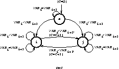
The DAG of the previous example has the following shape:
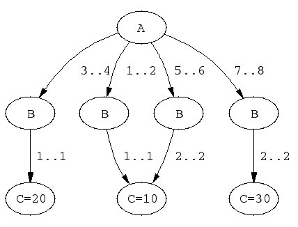
     
     
images/clpfd1.png
DAG corresponding to elts/3.

A couple of sample queries:

          | ?- elts(X, Y, Z).
          X in 1..8,
          Y in 1..2,
          Z in 10..30
          
          | ?- elts(X, Y, Z), Z #>= 15.
          X in(3..4)\/(7..8),
          Y in 1..2,
          Z in 20..30
          
          | ?- elts(X, Y, Z), Y = 1.
          Y = 1,
          X in 1..4,
          Z in 10..20
     

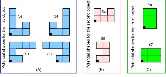
As an example with side constraints, consider assigning tasks to machines with given unavailibility periods. In this case, one can use a calendar constraint [CHIP 03, Beldiceanu, Carlsson & Rampon 05] to link the real origins of the tasks (taking the unavailibility periods into account) with virtual origins of the tasks (not taking the unavailibility periods into account). One can then state machine resource constraints using the virtual origins, and temporal constraints between the tasks using the real origins.

Assume, for example, three machines with unavailibility periods given by the following table:


images/clpfd3.png
Unavailibility periods for three machines.

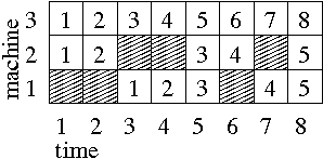
Machine 1 is not available during (real) time periods 1-2 and 6-6, machine 2 is not available during (real) time periods 3-4 and 7-7, and machine 3 is always available.

The following can then be used to express a calendar constraint for a given task scheduled on machine M in 1..3, with virtual origin V in 1..8, and real origin R in 1..8:

          calendar(M, V, R) :-
                  M in 1..3,
                  V in 1..8,
                  R in 1..8,
                  smt((M#=1 #/\ V in 1..3 #/\ R#=V+2) #\/
                      (M#=1 #/\ V in 4..5 #/\ R#=V+3) #\/
                      (M#=2 #/\ V in 1..2 #/\ R#=V) #\/
                      (M#=2 #/\ V in 3..4 #/\ R#=V+2) #\/
                      (M#=2 #/\ V in 5..5 #/\ R#=V+3) #\/
                      (M#=3               #/\ R#=V)).
     

or equivalently as:

          calendar(M, V, R) :-
              case(f(A,B,C),
                   [f(M,V,R)],
                   [node(0, A, [(1..1)-1, (2..2)-2, (3..3)-3]),
                    node(1, B, [(1..3)-[scalar_product([1,-1],[B,C],#=<,-2),
                                        scalar_product([1,-1],[C,B],#=<, 2)]-4,
                                (4..5)-[scalar_product([1,-1],[B,C],#=<,-3),
                                        scalar_product([1,-1],[C,B],#=<, 3)]-4]),
                    node(2, B, [(1..2)-[scalar_product([1,-1],[B,C],#=<, 0),
                                        scalar_product([1,-1],[C,B],#=<, 0)]-4,
                                (3..4)-[scalar_product([1,-1],[B,C],#=<,-2),
                                        scalar_product([1,-1],[C,B],#=<, 2)]-4,
                                (5..5)-[scalar_product([1,-1],[B,C],#=<,-3),
                                        scalar_product([1,-1],[C,B],#=<, 3)]-4]),
                    node(3, B, [(1..8)-[scalar_product([1,-1],[B,C],#=<, 0),
                                        scalar_product([1,-1],[C,B],#=<, 0)]-4]),
                    node(4, C, [(1..8)])]).
     

Note that equality must be modeled as the conjunction of inequalities, as only constraints of the form scalar_product(+Coeffs, +Xs, #=<, +Bound) are allowed as side constraints.

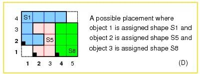
The DAG of the calendar constraint has the following shape:
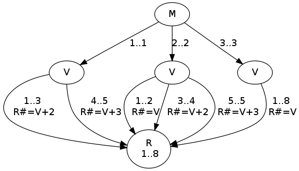
     
     
images/clpfd2.png
DAG corresponding to calendar/3.

A couple of sample queries:

          | ?- M in 1..3, V in 1..8, R in 1..8, calendar(M, V, R).
          M in 1..3,
          V in 1..8,
          R in 1..8
          
          | ?- M in 1..3, V in 1..8, R in 1..8, calendar(M, V, R), M #= 1.
          M = 1,
          V in 1..5,
          R in(3..5)\/(7..8)
          
          | ?- M in 1..3, V in 1..8, R in 1..8, calendar(M, V, R), M #= 2, V #> 4.
          M = 2,
          V = 5,
          R = 8
     

all_different(+Variables)
all_different(+Variables, +Options)
all_distinct(+Variables)
all_distinct(+Variables, +Options)
where Variables is a list of domain variables or integers. Each variable is constrained to take a value that is unique among the variables. Declaratively, this is equivalent to an inequality constraint for each pair of variables.

Options is a list of zero or more of the following:

consistency(Cons)
Which algorithm to use, one of the following:
domain
The default for all_distinct/[1,2] and assignment/[2,3]. an arc-consistency algorithm [Regin 94] is used, roughly linear in the total size of the domains. Implies on(dom).
bound
a bound-consistency algorithm [Mehlhorn 00] is used. This algorithm is nearly linear in the number of variables and values. Implies on(minmax).
value
The default for all_different/[1,2]. An algorithm achieving exactly the same pruning as a set of pairwise inequality constraints is used, roughly linear in the number of variables. Implies on(val).

on(On)
How eagerly to wake up the constraint. One of the following:
dom
(the default for all_distinct/[1,2] and assignment/[2,3]), to wake up when the domain of a variable is changed;
min
to wake up when the lower bound of a domain is changed;
max
to wake up when the upper bound of a domain is changed;
minmax
to wake up when some bound of a domain is changed;
val
(the default for all_different/[1,2]), to wake up when a variable becomes ground.

nvalue(?N, +Variables)
where Variables is a list of domain variables with finite bounds or integers, and N is an integer or a domain variable. True if N is the number of distinct values taken by Variables. Approximates bound-consistency in N and arc-consistency in Variables. Can be thought of as a relaxed version of all_distinct/2.

The following is a constraint over two lists of length n of variables. Each variable is constrained to take a value in [1,n] that is unique for its list. Furthermore, the lists are dual in a sense described below.

assignment(+Xs, +Ys)
assignment(+Xs, +Ys, +Options)
where Xs = [X1,...,Xn] and Ys = [Y1,...,Yn] are lists of domain variables or integers. True if all Xi, Yi in [1,n] and Xi=j iff Yj=i.

Options is a list of zero or more of the following, where Boolean must be true or false (false is the default):

on(On)
Same meaning as for all_different/2.
consistency(Cons)
Same meaning as for all_different/2.
circuit(Boolean)
If true, circuit(Xs,Ys) must hold for the constraint to be true.
cost(Cost,Matrix)
A cost is associated with the constraint and reflected into the domain variable Cost. Matrix should be an n*n matrix of integers, represented as a list of lists. The cost of the constraint is Matrix[1,X1]+...+Matrix[n,Xn].

With this option, an arc-consistency algorithm [Sellmann 02] is used, the complexity of which is roughly O(n(m + n log n)) where m is the total size of the domains.

The following constraint can be thought of as constraining n nodes in a graph to form a Hamiltonian circuit. The nodes are numbered from 1 to n. The circuit starts in node 1, visits each node, and returns to the origin.

circuit(+Succ)
circuit(+Succ, +Pred)
where Succ is a list of length n of domain variables or integers. The i:th element of Succ (Pred) is the successor (predecessor) of i in the graph. True if the values form a Hamiltonian circuit.

The following constraint can be thought of as constraining n tasks so that the total resource consumption does not exceed a given limit at any time. API change wrt. release 3:

cumulative(+Tasks)
cumulative(+Tasks,+Options)

A task is represented by a term task(Oi,Di,Ei,Hi,Ti) where Oi is the start time, Di the non-negative duration, Ei the end time, Hi the non-negative resource consumption, and Ti the task identifier. All fields are domain variables with bounded domains, or integers.

Let n be the number of tasks and L the global resource limit (by default 1, but see below), and:

          Hij = Hi, if Oi =< j < Oi+Di
          Hij = 0 otherwise
     

The constraint holds if:

  1. For every task i, Oi+Di=Ei, and
  2. For all instants j, H1j+...+Hnj =< L.

Options is a list of zero or more of the following, where Boolean must be true or false (false is the default).

limit(L)
See above.
precedences(Ps)
Ps encodes a set of precedence constraints to apply to the tasks. Ps should be a list of terms of the form:
               Ti-Tj #= Dij
          

where Ti and Tj should be task identifiers, and Dij should be a a domain variable (or an integer), denoting:

               Oi-Oj = Dij and Dij in r
          

global(Boolean)
if true, a more expensive algorithm will be used in order to achieve tighter pruning of the bounds of the parameters.

This constraint is due to Aggoun and Beldiceanu [Aggoun & Beldiceanu 93].

The following constraint can be thought of as constraining n tasks to be placed in time and on m machines. Each machine has a resource limit, which is interpreted as a lower or upper bound on the total amount of resource used on that machine at any point in time that intersects with some task.

cumulatives(+Tasks,+Machines)
cumulatives(+Tasks,+Machines,+Options)

A task is represented by a term task(Oi,Di,Ei,Hi,Mi) where Oi is the start time, Di the non-negative duration, Ei the end time, Hi the resource consumption (if positive) or production (if negative), and Mi a machine identifier. All fields are domain variables with bounded domains, or integers.

A machine is represented by a term machine(Mj,Lj) where Mj is the identifier and Lj is the resource bound of the machine. Both fields must be integers.

Let there be n tasks and:

          Hijm = Hi, if Mi=m and Oi =< j < Oi+Di
          Hijm = 0 otherwise
     

If the resource bound is lower (the default), the constraint holds if:

  1. For every task i, Si+Di=Ei, and
  2. For all machines m and instants j such that there exists a task i where Mi=m and Oi =< j < Oi+Di, H1jm+...+Hnjm >= Lm.

If the resource bound is upper, the constraint holds if:

  1. For every task i, Si+Di=Ei, and
  2. For all machines m and instants j, H1jm+...+Hnjm =< Lm.

Options is a list of zero or more of the following, where Boolean must be true or false (false is the default):

bound(B)
If lower (the default), each resource limit is treated as a lower bound. If upper, each resource limit is treated as an upper bound.
prune(P)
If all (the default), the constraint will try to prune as many variables as possible. If next, only variables that occur in the first nonground task term (wrt. the order given when the constraint was posted) can be pruned.
generalization(Boolean)
If true, extra reasoning based on assumptions on machine assignment will be done to infer more.
task_intervals(Boolean)
If true, extra global reasoning will be performed in an attempt to infer more.

The following constraint captures the relation between a list of values, a list of the values in ascending order, and their positions in the original list:

sorting(+Xs,+Ps,+Ys)
where Xs = [X1,...,Xn], Ps = [P1,...,Pn], and Ys = [Y1,...,Yn] are lists of domain variables or integers. The constraint holds if the following are true:

In practice, the underlying algorithm [Mehlhorn 00] is likely to achieve bound-consistency, and is guaranteed to do so if Ps is ground or completely free.

The following constraints model a set of lines or rectangles, respectively, so that no pair of objects overlap:

disjoint1(+Lines)
disjoint1(+Lines,+Options)
where Lines is a list of terms F(Sj,Dj) or F(Sj,Dj,Tj), Sj and Dj are domain variables with finite bounds or integers denoting the origin and length of line j respectively, F is any functor, and the optional Tj is an atomic term denoting the type of the line. Tj defaults to 0 (zero).

Options is a list of zero or more of the following, where Boolean must be true or false (false is the default):

decomposition(Boolean)
if true, an attempt is made to decompose the constraint each time it is resumed.
global(Boolean)
if true, a redundant algorithm using global reasoning is used to achieve more complete pruning.
wrap(Min,Max)
If used, the space in which the lines are placed should be thought of as a circle where positions Min and Max coincide, where Min and Max should be integers. That is, the space wraps around. Furthermore, this option forces the domains of the origin variables to be inside [Min,Max-1].
margin(T1,T2,D)
This option imposes a minimal distance D between the end point of any line of type T1 and the origin of any line of type T2. D should be a positive integer or sup. If sup is used, all lines of type T2 must be placed before any line of type T1.

This option interacts with the wrap/2 option in the sense that distances are counted with possible wrap-around, and the distance between any end point and origin is always finite.

The file library('clpfd/examples/bridge.pl') contains an example where disjoint1/2 is used for scheduling non-overlapping tasks.

disjoint2(+Rectangles)
disjoint2(+Rectangles,+Options)
where Rectangles is a list of terms F(Xj,Lj,Yj,Hj) or F(Xj,Lj,Yj,Hj,Tj), Xj and Lj are domain variables with finite bounds or integers denoting the origin and size of rectangle j in the X dimension, Yj and Hj are the values for the Y dimension, F is any functor, and the optional Tj is an atomic term denoting the type of the rectangle. Tj defaults to 0 (zero).

Options is a list of zero or more of the following, where Boolean must be true or false (false is the default):

decomposition(Boolean)
If true, an attempt is made to decompose the constraint each time it is resumed.
global(Boolean)
If true, a redundant algorithm using global reasoning is used to achieve more complete pruning.
wrap(Min1,Max1,Min2,Max2)
Min1 and Max1 should be either integers or the atoms inf and sup respectively. If they are integers, the space in which the rectangles are placed should be thought of as a cylinder wrapping around the X dimension where positions Min1 and Max1 coincide. Furthermore, this option forces the domains of the Xj variables to be inside [Min1,Max1-1].

Min2 and Max2 should be either integers or the atoms inf and sup respectively. If they are integers, the space in which the rectangles are placed should be thought of as a cylinder wrapping around the Y dimension where positions Min2 and Max2 coincide. Furthermore, this option forces the domains of the Yj variables to be inside [Min2,Max2-1].

If all four are integers, the space is a toroid wrapping around both dimensions.

margin(T1,T2,D1,D2)
This option imposes minimal distances D1 in the X dimension and D2 in the Y dimension between the end point of any rectangle of type T1 and the origin of any rectangle of type T2. D1 and D2 should be positive integers or sup. If sup is used, all rectangles of type T2 must be placed before any rectangle of type T1 in the relevant dimension.

This option interacts with the wrap/4 option in the sense that distances are counted with possible wrap-around, and the distance between any end point and origin is always finite.

synchronization(Boolean)
Let the assignment dimension and the temporal dimension denote the two dimensions, no matter which is the X and which is the Y dimension. If Boolean is true, a redundant algorithm is used to achieve more complete pruning for the following case:
  • All rectangles have size 1 in the assignment dimension.
  • Some rectangles have the same origin and size in the temporal dimension, and that origin is not yet fixed.

The following example shows an artificial placement problem involving 25 rectangles including four groups of rectangles whose left and right borders must be aligned. If Synch is true, it can be solved with first-fail labeling in 23 backtracks. If Synch is false, 60 million backtracks do not suffice to solve it.

               ex([O1,Y1a,Y1b,Y1c,
                   O2,Y2a,Y2b,Y2c,Y2d,
                   O3,Y3a,Y3b,Y3c,Y3d,
                   O4,Y4a,Y4b,Y4c],
                  Synch) :-
                       domain([Y1a,Y1b,Y1c,
                               Y2a,Y2b,Y2c,Y2d,
                               Y3a,Y3b,Y3c,Y3d,
                               Y4a,Y4b,Y4c], 1, 5),
                       O1 in 1..28,
                       O2 in 1..26,
                       O3 in 1..22,
                       O4 in 1..25,
                       disjoint2([t(1,1,5,1),    t(20,4,5,1),
                                  t(1,1,4,1),    t(14,4,4,1),
                                  t(1,2,3,1),    t(24,2,3,1),
                                  t(1,2,2,1),    t(21,1,2,1),
                                  t(1,3,1,1),    t(14,2,1,1),
                                  t(O1,3,Y1a,1),
                                  t(O1,3,Y1b,1),
                                  t(O1,3,Y1c,1),
                                  t(O2,5,Y2a,1),
                                  t(O2,5,Y2b,1),
                                  t(O2,5,Y2c,1),
                                  t(O2,5,Y2d,1),
                                  t(O3,9,Y3a,1),
                                  t(O3,9,Y3b,1),
                                  t(O3,9,Y3c,1),
                                  t(O3,9,Y3d,1),
                                  t(O4,6,Y4a,1),
                                  t(O4,6,Y4b,1),
                                  t(O4,6,Y4c,1)],
                                 [synchronization(Synch)]).
          

geost(+Objects,+Shapes)
geost(+Objects,+Shapes,+Options)
geost(+Objects,+Shapes,+Options,+Rules)
constrains the location in space of non-overlapping multi-dimensional Objects, each of which taking a shape among a set of Shapes.

Each shape is defined as a finite set of shifted boxes, where each shifted box is described by a box in a k-dimensional space at the given offset with the given sizes. A shifted box is described by a ground term sbox(Sid,Offset,Size) where Sid, an integer, is the shape id; Offset, a list of k integers, denotes the offset of the shifted box from the origin of the object; and Size, a list of k integers greater than zero, denotes the size of the shifted box. Then, a shape is a collection of shifted boxes all sharing the same shape id. The shifted boxes associated with a given shape must not overlap. Shapes is thus the list of such sbox/3 terms.

Each object is described by a term object(Oid,Sid,Origin where Oid, an integer, is the unique object id; Sid, an integer or domain variable, is the shape id; and Origin, a list of integers or domain variables, is the origin coordinate of the object. If Sid is nonground, the object is said to be polymorphic. The possible values for Sid are the shape ids that occur in Shapes. Objects is thus the list of such object/3 terms.

If given, Options is a list of zero or more of the following, where Boolean must be true or false (false is the default):

lex(ListOfOid)
where ListOfOid should be a list of distinct object ids, denotes that the origin vectors of the objects according to ListOfOid should be in ascending lexicographic order. Multiple lex/1 options can be given, but should mention disjoint sets of objects.
cumulative(Boolean)
If true, redundant reasoning methods are enabled, based on projecting the objects onto each dimension.
disjunctive(Boolean)
If true, cliques of objects are detected that clash in one dimension and so must be separated in the other dimension. This method only applies in the 2D case.
longest_hole(Value,Maxbacks)
This method only applies in the 2D case and in the absence of polymorphic objects. Value can be all, true or false. If true, the filtering algorithm computes and uses information about holes that can be tolerated without necessarily failing the constraint. If all, more precise information is computed. If false, no such information is computed. Maxbacks should be an integer >= -1 and gives a bound on the effort spent tightening the longest hole information. Experiments suggest that 1000 may be a reasonable compromise value.
parconflict(Boolean)
If true, redundant reasoning methods are enabled, based on computing the number of items that can be put in parallel in the different dimensions.
visavis_init(Boolean)
If true, a redundant method is enabled that statically detects placements that would cause too large holes. This method can be quite effective.
visavis_floating(Boolean)
If true, a redundant method is enabled that dynamically detects placements that would cause too large holes. It's more general than the following option, but only applies in the 2D case and in the absence of polymorphic objects. This method has been shown to pay off only in rare cases.
visavis(Boolean)
If true, a redundant method is enabled that dynamically detects placements that would cause too large holes. This method has not been shown to pay off experimentally.
corners(Boolean)
If true, a redundant method is enabled that reasons in terms on borders that impinge on the corners of objects. This method only applies in the 2D case. It has not been shown to pay off experimentally.
task_intervals(Boolean)
If true, a redundant reasoning method is enabled that detects overcrowded and undercrowded regions of the placement space. This method has not been shown to pay off experimentally.
dynamic_programming(Boolean)
If true, a redundant reasoning method is enabled that solves a 2D knapsack problem for every two adjacent columns of the projection of the objects onto each dimension. This method has pseudo-polynomial complexity but can be quite powerful.
polymorphism(Boolean)
If true, a reasoning method is enabled that is relevant in the context of polymorphic objects and no slack. The method detects parts of the placement space that cannot be filled and thus fails the constraint. This method has not been shown to pay off experimentally.
pallet_loading(Boolean)
If true, and if all objects consist of a single shifted box of the same shape, modulo rotations, a redundant method is enabled that recognizes necessary conditions for this special case.
overlap(Boolean)
If true, the constraint that objects be non-overlapping is lifted. This option is useful mainly in conjunction with the Rules argument, in case the placement of objects should be restricted by the Rules only.
volume(Total)
If given, Total is constrained to be the total volume of Objects.
bounding_box(Lower,Upper)
Lower=[L1,...,Lk] and Upper=[U1,...,Uk] should be lists of integers or domain variables. The following conditions are imposed:
  • For every point P = [P1,...,Pk] occupied by an object, L1 =< P1 < U1, ..., Lk =< Pk < Uk.
  • For every j in 1..k, there exists a point P = [P1,...,Pj,...,Pk] occupied by an object such that Pj=Lj.
  • For every j in 1..k, there exists a point P = [P1,...,Pj,...,Pk] occupied by an object such that Pj=Uj-1.

fixall(Flag,Patterns)
If given, Flag is an integer or domain variable in 0..1. If Flag equals 1, either initially or by binding Flag during search, the constraint switches behavior into greedy assignment mode. The greedy assignment will either succeed and assign all shape ids and origin coordinates to values that satisfy the constraint, or merely fail. Flag is never bound by the constraint; its sole function is to control the behavior of the constraint.

Greedy assignment is done one object at a time, in the order of Objects. The assignment per object is controlled by Patterns, which should be a list of one or more pattern terms of the form object(_,SidSpec,OriginSpec), where SidSpec is a term min(I) or max(I), OriginSpec is a list of k such terms, and I is a unique integer between 1 and k+1.

The meaning of the pattern is as follows. The variable in the position of min(1) or max(1) is fixed first; the variable in the position of min(2) or max(2) is fixed second; and so on. min(I) means trying values in ascending order; max(I) means descending order.

If Patterns contains m pattern, then object 1 is fixed according to pattern 1, ..., object m is fixed according to pattern m, object m+1 is fixed according to pattern 1, and so on. For example, suppose that the following option is given:

               fixall(F, [object(_,min(1),[min(3),max(2)]),
                          object(_,max(1),[min(2),max(3)])])
          

Then, if the program binds F to 1, the constraint enters greedy assignment mode and endeavors to fix all objects as follows.

  • For object 1, 3, ..., (a) the shape is fixed to the smallest possible value, (b) the Y coordinate is fixed to the largest possible value, (c) the X coordinate is fixed to the smallest possible value.
  • For object 2, 4, ..., (a) the shape is fixed to the largest possible value, (b) the X coordinate is fixed to the smallest possible value, (c) the Y coordinate is fixed to the largest possible value.

If given, Rules is a list of zero or more terms of the form shown below, and impose extra constraints on the placement of the objects. For the time being, the details are described in [Carlsson, Beldiceanu & Martin 08]. Please note: the rules require that all shapes of a polymorphic objects consist of the same number of shifted boxes. For example, Shapes = [sbox(1,[0,0],[3,1]),sbox(1,[0,1],[2,4]),sbox(2,[0,0],[3,1])] will not work.

sentence ::= macro | fol

macro ::= head ---> body

head ::= term { to be substituted by a body }

body ::= term { to substitute for a head }

fol ::= #\ fol { negation }
| fol #/\ fol { conjunction }
| fol #\/ fol { disjunction }
| fol #=> fol { implication }
| fol #<=> fol { equivalence }
| exists(var,collection,fol) { existential quantification }
| forall(var,collection,fol) { universal quantification }
| card(var,collection,integer,integer,fol) { cardinality }
| true
| false
| expr relop expr { rational arithmetic }
| head { macro application }

expr ::= expr + expr
| - expr
| expr - expr
| min(expr,expr)
| max(expr,expr)
| expr * groundexpr
| groundexpr * expr
| expr / groundexpr
| attref
| integer
| fold(var,collection,fop,expr,expr)
| variable { quantified variable }
| head { macro application }

groundexpr ::= expr { where expr is ground }

attref ::= entity ^ attr

attr ::= term { attribute name }
| variable { quantified variable }

relop ::= #< | #= | #> | #\= | #=< | #>=

fop ::= + | min | max

collection ::= list
| objects(list) { list of oids }
| sboxes(list) { list of sids }

The following example shows geost/2 modeling three non-overlapping objects. The first object has four possible shapes, and the other two have two possible shapes each.

          ?- domain([X1,X2,X3,Y1,Y2,Y3], 1, 4),
             S1 in 1..4,
             S2 in 5..6,
             S3 in 7..8,
             geost([object(1,S1,[X1,Y1]),
                    object(2,S2,[X2,Y2]),
                    object(3,S3,[X3,Y3])],
                   [sbox(1,[0,0],[2,1]),
                    sbox(1,[0,1],[1,2]),
                    sbox(1,[1,2],[3,1]),
                    sbox(2,[0,0],[3,1]),
                    sbox(2,[0,1],[1,3]),
                    sbox(2,[2,1],[1,1]),
                    sbox(3,[0,0],[2,1]),
                    sbox(3,[1,1],[1,2]),
                    sbox(3,[2,2],[3,1]),
                    sbox(4,[0,0],[3,1]),
                    sbox(4,[0,1],[1,1]),
                    sbox(4,[2,1],[1,3]),
                    sbox(5,[0,0],[2,1]),
                    sbox(5,[1,1],[1,1]),
                    sbox(5,[0,2],[2,1]),
                    sbox(6,[0,0],[3,1]),
                    sbox(6,[0,1],[1,1]),
                    sbox(6,[2,1],[1,1]),
                    sbox(7,[0,0],[3,2]),
                    sbox(8,[0,0],[2,3])]).
     

The shapes are illustrated in the following picture:


images/geost1a.png
geost/2: three objects and eight shapes

A ground solution is shown in the following picture:


images/geost1b.png
geost/2: a ground solution

The following example shows how to encode in Rules “objects with oid 1, 2 and 3 must all be at least 2 units apart from objects with oid 4, 5 and 6”.

          [ (origin(O1,S1,D) ---> O1^x(D)+S1^t(D))),
          
            (end(O1,S1,D) ---> O1^x(D)+S1^t(D)+S1^l(D)),
          
            (tooclose(O1,O2,S1,S2,D) --->
                end(O1,S1,D)+2 #> origin(O2,S2,D) #/\
                end(O2,S2,D)+2 #> origin(O1,S1,D)),
          
            (apart(O1,O2) --->
                forall(S1,sboxes([O1^sid]),
                    forall(S2,sboxes([O2^sid]),
                        #\ tooclose(O1,O2,S1,S2,1) #\/
                        #\ tooclose(O1,O2,S1,S2,2)))),
          
            (forall(O1,objects([1,2,3]),
                forall(O2,objects([4,5,6]), apart(O1,O2))))].
     

The following example shows how to encode in Rules “objects 3 and 7 model rooms that must be adjacent and have a common border at least 1 unit long”.

          [ (origin(O1,S1,D) ---> O1^x(D)+S1^t(D))),
          
            (end(O1,S1,D) ---> O1^x(D)+S1^t(D)+S1^l(D)),
          
            (overlap(O1,S1,O2,S2,D) --->
                end(O1,S1,D) #> origin(O2,S2,D) #/\
                end(O2,S2,D) #> origin(O1,S1,D)),
          
            (abut(O1,O2) --->
                forall(S1,sboxes([O1^sid]),
                    forall(S2,sboxes([O2^sid]),
                        ((origin(O1,S1,1) #= end(O2,S2,1) #\/
                          origin(O2,S2,1) #= end(O1,S1,1)) #/\
                         overlap(O1,S1,O2,S2,2)) #\/
                        ((origin(O1,S1,2) #= end(O2,S2,2) #\/
                          origin(O2,S2,2) #= end(O1,S1,2)) #/\
                         overlap(O1,S1,O2,S2,1))))),
          
            (forall(O1,objects([3]),
                forall(O2,objects([7]), abut(O1,O2))))].
     

The following constraints express the fact that several vectors of domain variables are in ascending lexicographic order:

lex_chain(+Vectors)
lex_chain(+Vectors,+Options)
where Vectors is a list of vectors (lists) of domain variables with finite bounds or integers. The constraint holds if Vectors are in ascending lexicographic order.

Options is a list of zero or more of the following:

op(Op)
If Op is the atom #=< (the default), the constraints holds if Vectors are in non-descending lexicographic order. If Op is the atom #<, the constraints holds if Vectors are in strictly ascending lexicographic order.
increasing
This option imposes the additional constraint that each vector in Vectors be sorted in strictly ascending order.
among(Least,Most,Values)
If given, Least and Most should be integers such that 0 =< Least =< Most and Values should be a list of distinct integers. This option imposes the additional constraint on each vector in Vectors that at least Least and at most Most elements belong to Values.

Unless the increasing/0 or among/3 options are given, the underlying algorithm [Carlsson & Beldiceanu 02] guarantees arc-consistency.

The following constraint provides a general way of defining any constraint involving sequences whose checker, i.e. a procedure that classifies ground instances as solutions or non-solutions, can be expressed by a finite automaton, deterministic or nondeterministic, extended with counter operations on its arcs. The point is that it is very much easier to come up with such a checker than to come up with a filtering algorithm for the constraint of interest.

automaton(Signature, SourcesSinks, Arcs)
automaton(Sequence, Template, Signature, SourcesSinks, Arcs, Counters, Initial, Final)
automaton(Sequence, Template, Signature, SourcesSinks, Arcs, Counters, Initial, Final, Options)
The arguments are described below in terms of their abstract syntax:
Sequence
The sequence of terms of interest; abstract grammar category sequence.
Template
A template for an item of the sequence; abstract grammar category template. Only relevant if some state transition involving counter arithmetic mentions a variable occurring in Template, in which case the corresponding term in a sequence element will be accessed.
Signature
The signature of Sequence; abstract grammar category signature. The automaton is not driven by Sequence itself, but by Signature, which ranges over some alphabet, implicitly defined by the values used by Arcs. In addition to automaton/[8,9], you must call a constraint that maps Sequence to Signature.
SourcesSinks
The source and sink nodes of the automaton; abstract grammar category sourcessinks.
Arcs
The arcs (transitions) of the automaton; abstract grammar category arcs. Any transition not mentioned is assumed to go to an implicit failure node. An arc optionally contains expressions for updated counter values; by default, the counters remain unchanged. Conditional updates can be specified.
Counters
A list of variables, local to the constraint; abstract grammar category counters.
Initial
A list of initial values, usually instantiated; abstract grammar category initial.
Final
A list of final values, usually uninstantiated; abstract grammar category final.
Options
Abstract grammar category options; a list of zero or more of the following terms. All but the last option are implemented by adding auxiliary counters to the automaton including the necessary updates in the arcs:
valueprec(First,Later,N)
N is unified with n, computed such that: if the value Later occurs in the Signature, First occurs n times before the first occurrence of Later, otherwise n=0.
anystretchocc(N)
N is unified with the number of (nonempty) stretches of any single value in the Signature.
stretchocc(ValuePat,N)
N is unified with the number of stretches of values matching ValuePat (abstract grammar category valuepat) in the Signature.
stretchoccmod(ValuePat,Mod,N)
N is unified with the number (modulo Mod) of stretches of values matching ValuePat (abstract grammar category valuepat) the Signature.
stretchmaxlen(ValuePat,N)
N is unified with n, computed such that: if values matching ValuePat (abstract grammar category valuepat) occur the Signature, n is the length of the longest such stretch, otherwise n=0.
stretchminlen(ValuePat,N)
N is unified with n, computed such that: if values matching ValuePat (abstract grammar category valuepat) occur the Signature, n is the length of the shortest such stretch, otherwise n is a large integer.
wordocc(WordPat,N)
N is unified with the number of words matching WordPat (abstract grammar category wordpat) in the Signature.
wordoccmod(WordPat,Mod,N)
N is unified with the number (modulo Mod) of words matching WordPat (abstract grammar category wordpat) in the Signature.
wordprefix(WordPat,ZO)
If the prefix of the Signature matches WordPat (abstract grammar category wordpat), ZO is unified with 1, otherwise with 0.
wordsuffix(WordPat,ZO)
If the suffix of the Signature matches WordPat (abstract grammar category wordpat), ZO is unified with 1, otherwise with 0.
state(Map,StateVars)
For a signature of length k, the constraint is implemented by decomposition into k smaller constraints mapping an old state to a new state. The states are represented as domain variables. StateVars forms the list of these k+1 domain variables, starting with the initial state and ending with the final state. Map gives the interpretation of their values: it is a list of pairs Node-Value such that if the nth state variable Sn equals Value, then the automaton is in state Node having read n symbols.

Abstract syntax:

sequence ::= list of template {all of which of the same shape}

template ::= term {most general shape of the sequence}
{its variables should be local to the constraint}

signature ::= list of variable

sourcessinks ::= list of nodespec

nodespec ::= source(node) {an initial state}
| sink(node) {an accept state}

node ::= term

arcs ::= list of arc

arc ::= arc(node,integer,node) {from node, integer, to node}
| arc(node,integer,node,exprs){exprs correspond to new counter values}
| arc(node,integer,node,conditional)

conditional ::= (cond -> exprs)
| (conditional ; conditional)

exprs ::= list of Expr {of same length as counters}
{Expr as defined in Syntax of Arithmetic Expressions}
{over counters, template and constants}
{variables occurring in counters correspond to old counter values}
{variables occurring in template refer to the current element of sequence}

cond ::= constraint {over counters, template and constants}
{must be reifiable or true}

counters ::= list of variable {should be local to the constraint}

initial ::= list of dvar {of same length as counters}

final ::= list of dvar {of same length as counters}

option ::= state(list of term,list of dvar)
| valueprec(integer,integer,dvar)
| anystretchocc(dvar)
| stretchocc(valuepat,dvar)
| stretchoccmod(valuepat,dvar,integer)
| stretchmaxlen(valuepat,dvar)
| stretchminlen(valuepat,dvar)
| wordocc(wordpat,dvar)
| wordoccmod(wordpat,dvar,integer)
| wordprefix(wordpat,dvar)
| wordsuffix(wordpat,dvar)

valuepat ::= integer
| list of integer {alternatives}
| valuepat/valuepat {alternatives}

wordpat ::= list of valuepat

dvar ::= variable or integer

If no counters are used, the arguments Counters, Initial and Final should be []. The arguments Template and Sequence are only relevant if some Expr mentions a variable in Template, in which case the corresponding position in Sequence will be used at that point.

The constraint holds for a ground instance Sequence if:

Here is an example. Suppose that you want to define the predicate inflexion(N,L,Opt) which should hold if L is a list of domain variables, and N is the number of times that the sequence order switches between strictly increasing and strictly decreasing. For example, the sequence [1,1,4,8,8,2,7,1] switches order three times.

Such a constraint is conveniently expressed by a finite automaton over the alphabet [<,=,>] denoting the order between consecutive list elements. A counter is incremented when the order switches, and is mapped to the first argument of the constraint. The automaton could look as follows:


images/inflexion2.png
Automaton for inflexion/3

The following piece of code encodes this using automaton/9. The auxiliary predicate inflexion_signature/2 maps the sequence to a signature where the consecutive element order is encoded over the alphabet [0,1,2]. We use one counter with initial value 0 and final value N (an argument of inflexion/3). Two transitions increment the counter. All states are accept states.

          inflexion(N, Vars, Opt) :-
                  inflexion_signature(Vars, Sign),
                  automaton(Sign, _, Sign,
                            [source(s),sink(i),sink(j),sink(s)],
                            [arc(s,1,s      ),
                             arc(s,2,i      ),
                             arc(s,0,j      ),
                             arc(i,1,i      ),
                             arc(i,2,i      ),
                             arc(i,0,j,[C+1]),
                             arc(j,1,j      ),
                             arc(j,0,j      ),
                             arc(j,2,i,[C+1])],
                            [C],[0],[N],Opt).
          
          inflexion_signature([], []).
          inflexion_signature([_], []) :- !.
          inflexion_signature([X,Y|Ys], [S|Ss]) :-
                  S in 0..2,
                  X #> Y #<=> S #= 0,
                  X #= Y #<=> S #= 1,
                  X #< Y #<=> S #= 2,
                  inflexion_signature([Y|Ys], Ss).
     

Some queries:

          /* count the #inflections of a ground string */
          | ?- inflexion(N, [1,1,4,8,8,2,7,1], []).
          N = 3 ? <RET>
          yes
     
          /* find strings with two inflections */
          | ?- length(L,4), domain(L,0,1), inflexion(2,L,[]), labeling([],L).
          L = [0,1,0,1] ? ;
          L = [1,0,1,0] ? ;
          no
     
          /* find strings that are strictly increasing, strictly decreasing or all equal */
          | ?- length(L,4), domain(L,0,3), inflexion(I,L,[anystretchocc(1)]), labeling([],L).
          I = 0,
          L = [0,0,0,0] ? ;
          I = 0,
          L = [0,1,2,3] ? ;
          I = 0,
          L = [1,1,1,1] ? ;
          I = 0,
          L = [2,2,2,2] ? ;
          I = 0,
          L = [3,2,1,0] ? ;
          I = 0,
          L = [3,3,3,3] ? ;
          no
     
          /* find strings that contain an increase followed by a decrease */
          | ?- length(L,4), domain(L,0,1), inflexion(I,L,[wordocc([2,0],1)]), labeling([],L).
          I = 1,
          L = [0,0,1,0] ? ;
          I = 1,
          L = [0,1,0,0] ? ;
          I = 2,
          L = [0,1,0,1] ? ;
          I = 2,
          L = [1,0,1,0] ? ;
          no
     

This constraint uses techniques from [Beldiceanu, Carlsson & Petit 04] and [Beldiceanu, Carlsson, Flener & Pearson 10].


Send feedback on this subject.